Fig.4: larger. Klong
Fig.5: larger. Klong
| Prev: Basic Statistical Functions | Content | Next: χ2 Tests |
The Klong nstat module contains a set of functions
implementing some selected discrete and continuous
probability distributions.
For instance,
n.pdf is the
probability density function
(PDF) of the
normal distribution.
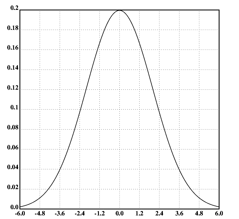
Probability functions can be plotted using the interactive
plotter interface (the result is the scaling of the y-axis; see fig.4 for
the plot):
v.aplot(n.pdf(;0;4);-6;6)
|
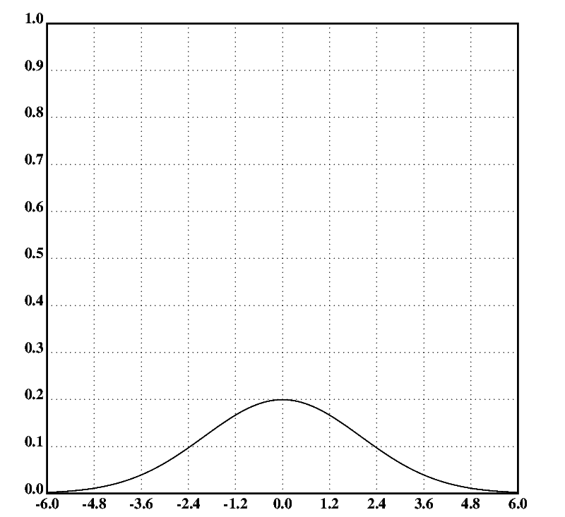
To display the graph in a more familiar frame with a y-axis ranging
from zero to one, the y-axis is adjusted using the set.y
function, specifying the origin, the limit, and the scaling step width
of the axis. The vp function re-plots the most recently
plotted graph, using the new parameters. Fig.5 shows the adjusted plot.
    set.y(0;1;0.1)
    vp()
|
While the interactive plotter interface is useful for quickly plotting
graphs of data sets and functions, there are sometimes good reasons for
using the nplot functions directly. For example, they can
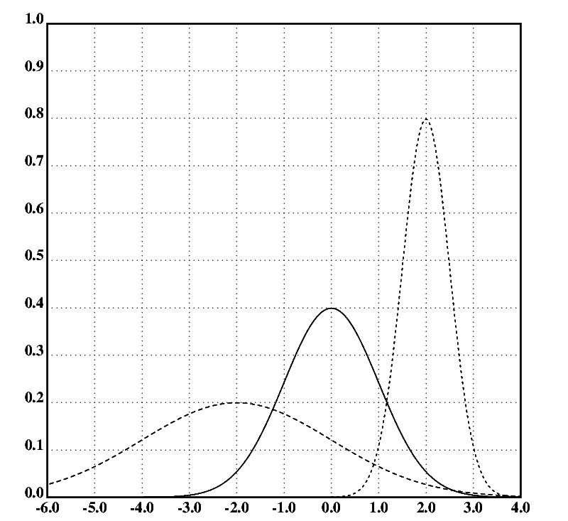
The nplot functions always write Postscript code to the
output channel; they never display the generated panels. Hence they are
more suitable for batch processing than interactive use. Here are the
nplot instructions for plotting normal distribution curves
with different parameters in different line styles:
    grid([-6 4 1];[0 1 0.1])
    plot(n.pdf(;0;1))
    setline(1);plot(n.pdf(;-2;4))
    setline(2);plot(n.pdf(;2;0.25))
    draw()
|
The output of the program can then be viewed with a Postscript viewer or converted to an image file format. The panel generated by the above program can be found in fig.6. A commented version of the above program is linked below the figure.
The signature of the n.pdf function is
n.pdf(x;μ;σ2), where x is
the
score
whose probability is to be computed, μ is the mean and
σ2 the variance of the distribution. There are some other
functions dealing with the normal distribution. They all have a
n. prefix attached to their names. These functions include
the
probability density function,
the
cumulative distribution function
(CDF), the
mean
and
variance,
and the
skewness:
n.pdf(0;0;4)
|
These functions are also available for all other probability distributions
supported by nstat. Discrete probability distributions,
however, have a
probability mass function
(PMF) instead of a
density function. The continuous distributions also include a
quantile function
(QF), which is the inverse function of the CDF. Here is a summary
of the supported distributions and the signatures of the corresponding
functions:
| Distribution | Prefix | PMF/PDF | CDF | μ | σ2 | Skew | QF |
|---|---|---|---|---|---|---|---|
| Frequency * | f. | pmf(x;F) | cdf(x;F) | mu(F) | var(F) | -/- | -/- |
| Uniform (discrete) |
u. | pmf(x;a;b) | cdf(x;a;b) | mu(a;b) | var(a;b) | skew(a;b) | -/- |
| Geometric | geo. | pmf(x;p) | cdf(x;p) | mu(p) | var(p) | skew(p) | -/- |
| Binomial | b. | pmf(x;n;p) | cdf(x;n;p) | mu(n;p) | var(n;p) | skew(n;p) | -/- |
| Hypergeometric | hyp. | pmf(x;n,p,N) | cdf(x;n,p,N) | mu(n;p;N) | var(n;p;N) | skew(n;p;N) | -/- |
| Poisson | poi. | pmf(x;λ) | cdf(x;λ) | mu(λ) | var(λ) | skew(λ) | -/- |
| Normal | n. | pdf(x;μ;σ2) | cdf(x;μ;σ2) | mu(μ;σ2) | var(μ;σ2) | skew(μ;σ2) | qf(p;μ;σ2) |
| Standard Normal |
ndf(x) | cdf(x) phi(x) |
0 | 1 | 0 | qf(p) | |
| Lognormal | ln. | pdf(x;μ;σ2) | cdf(x;μ;σ2) | mu(μ;σ2) | var(μ;σ2) | skew(μ;σ2) | qf(p;μ;σ2) |
| χ2 | x2. | pdf(ν;x) | cdf(ν;x) | mu(ν) | var(ν) | skew(ν) | qf(ν;p) |
| Student's t | t. | pdf(ν;x) | cdf(ν;x) | mu(ν) | var(ν) | skew(ν) | qf(ν;p) |
* The F parameter in the frequency distribution
functions indicates a frequency distribution of the form
[[value frequency] ...].
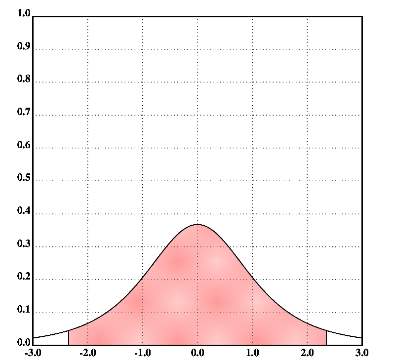
The interactive plotter contains functions for highlighting areas under
the graphs of probability functions. They can be used, for example, to
illustrate
confidence intervals
and
critical regions.
For instance, a 90% confidence interval under a
t-distribution
curve
with ν=3
degrees of freedom
can be plotted as follows using the vplot interface:
    set.x(-3;3;1)
    set.y(0;1;0.1)
    t::t.qf(3;0.95)
    set.fill(-t;t;0)
    v.plot(t.pdf(3;))
|
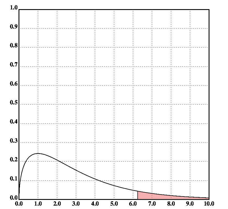
The output will look similar to that to fig.7. Fig.8 shows an
α=0.1 critical region in a χ2 distribution
with ν=3. For Klong code
using the nplot interface, see the programs linked
in under the figures.
| Prev: Basic Statistical Functions | Content | Next: χ2 Tests |