An Introduction to
Statistics with Klong

Non-Linear Regression

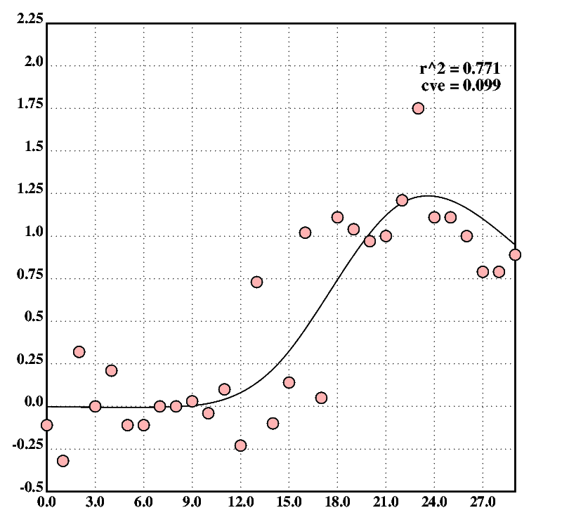
Here is a non-linear data set (again, the actual set may be different due to the random error, if you want to get the same results, do not use the formula, but copy-paste the array instead):

    X::rndn(;2)'err(10;1.5;dist(cdf;30;[-5 5])%30)
[-0.11 -0.32  0.32 0.0   0.21 -0.11
 -0.11  0.0   0.0  0.03 -0.04  0.1
 -0.23  0.73 -0.1  0.14  1.02  0.05
  1.11  1.04  0.97 1.0   1.21  1.75
  1.11  1.11  1.0  0.79  0.79  0.89]

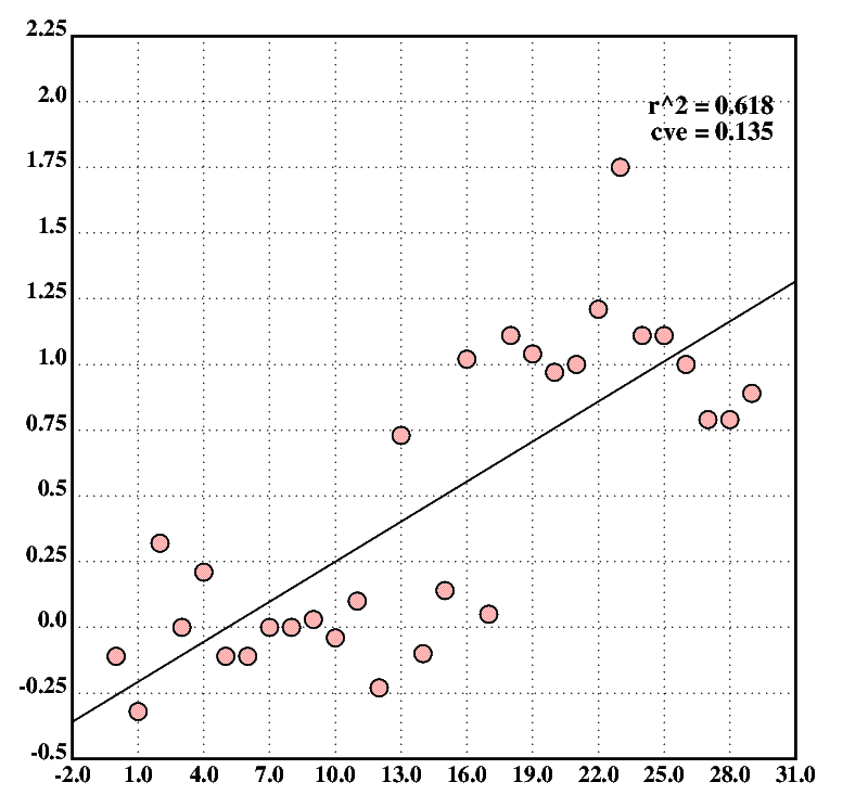
We can then turn the data set into an x/y set and scatter-plot it. The plot in fig.11, showing the regression line, suggests a non-linear relationship between the variables. The code also computes and prints the r² value and the cross validation error (CVE) for the model.

    XY::(!30),'X 
    L::lreg(XY)
    plot(lr(;L))
    scplot2(XY)
    desc0("r^2 = ",$rndn(r2(XY;lr(;L));3))
    desc1("cve = ",$rndn(cve(lreg;lr;XY);3))       

Fig.11: larger. Klong

A natural cubic spline through a data set can be created with the spl function of the nstat module. The function creates a histogram of k bars, where each bar indicates the mean of the values covered by it. The created spline then has k degrees of freedom and goes through the values indicated by the histogram.

Fig.12: larger. Klong

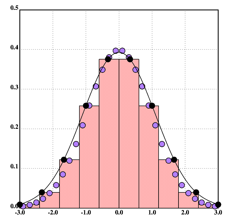
Fig.12 shows a normally distributed data set (purple dots), a histogram, and a spline with ten degrees of freedom approximating the distribution of the data points (black). The knots of the spline show as black dots. (You may have to zoom into the image to see the colors.) The figure is created as follows (omitting style instructions, see the program linked under the figure for the full code):

    F::freq(ndf;30;[-3 3])
    df::10
    barplot(hist(df;F))
    scplot(F)
    S::spl(df;((!#F)%29%6)-3),'F
    plot(sp(;S))
    scplot2(S)

Like in the linear regression model, there is a fitting function (spl) and a predicting function (sp). spl takes the degrees of freedom and the data set as values, and sp expects a value of the independent variable and a spline delivered by spl.

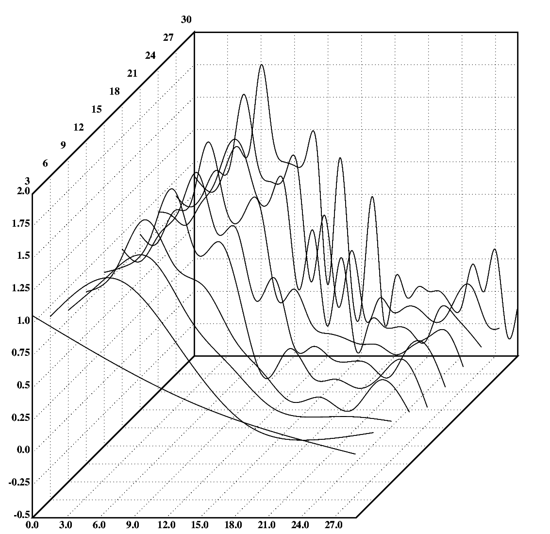
The following Klong instructions plot a set of splines through the data set in fig.11 as a 3D-plot. The chosen splines have 3,6,...,30 degrees of freedom. The plot is shown in fig.13. Note that the spline plots are mirrored across the x-axis in the figure to improve the visual effect. (Again, the full program, including the mirroring, is linked under the figure.)

    k::3+3*!10
    cgrid3(0,((#XY)-1),3;[-0.5 2.0 0.25];k)
    S::spl(;XY)'k
    plot3(sp(;S@y))

Fig.13: larger. Klong
Fig.14: larger. Klong

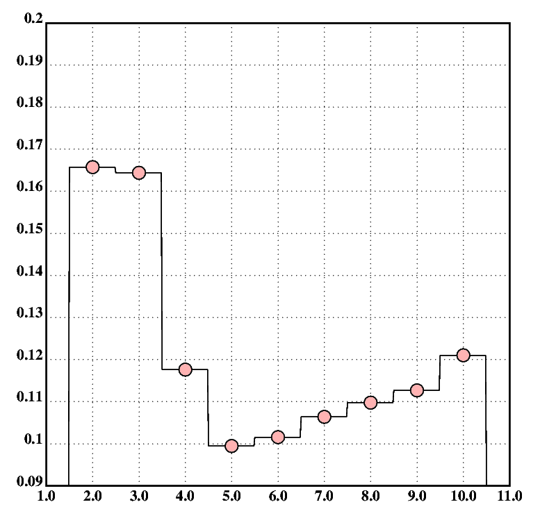
The cross validation errors (CVEs) corresponding to the splines plotted in fig.13 are shown in fig.14. Lower values indicate a better fit of the model to the data. The CVE data set is computed as follows (values are round to two decimal places):

    {[k];k::x;cve(spl(k;);sp2;XY)}'3+3*!10
[0.16 0.1 0.11 0.11 0.13 0.12 0.15 0.16 0.17 0.21]

The cve function performs Leave One Out cross validation (LOOCV) on a data set and model and returns the resulting error (CVE). The parameters of cve are: a model fitting function, a predicting function, and an x/y set. Note that sp2 is used instead of sp for prediction; it will extrapolate a result, if its argument is not covered by the spline.

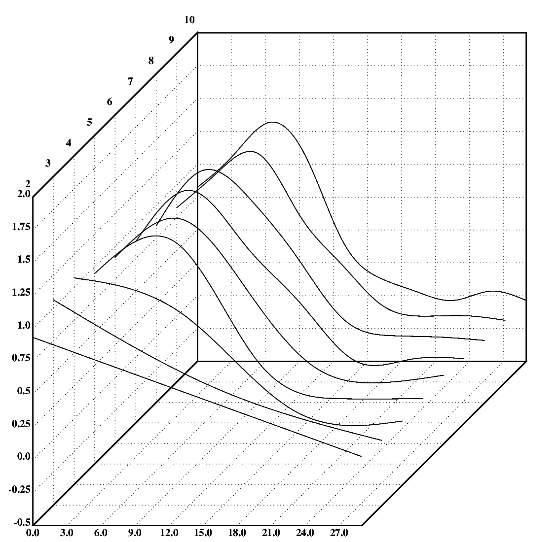
Because there is a valley around six degrees of freedom (DF), it makes sense to examine the splines up 10 DF more closely. So, for your entertainment, here are figs.15 and 16, showing these splines and the corresponding CVE values.

Fig.15: larger. Klong
Fig.16: larger. Klong

The final panel (fig.17) shows the non-linear model with the least CVE, a spline with five degrees of freedom, and the corresponding r² and CVE values.

Fig.17: larger. Klong

contact  |  privacy